Intraday heatmap

This example shows how to visualise solar irradiance as a time-of-day vs. date heatmap using solarpy.plotting.plot_intraday_heatmap().

Basic usage

sphinx_gallery_thumbnail_number = 2

Read a year of 1-minute GHI measurements and plot them as a heatmap.

import solarpy

data, meta = solarpy.iotools.read_t16(
    "https://raw.githubusercontent.com/AssessingSolar/solarpy/refs/heads/main/data/LYN_2023.csv",  # noqa: E501
    map_variables=True,
)

fig, ax = solarpy.plotting.plot_intraday_heatmap(
    time=data.index,
    values=data["ghi"],
    colorbar_label="GHI [W/m²]",
    time_resolution=1,  # frequency of timesteps in minutes
)
fig.tight_layout()

Heat maps are particularly useful for visualising data, as all data points are distinctly visible, unlike in line or scatter plots where overlapping data points is common.

However, the colormap used in the above plot (viridis), is not ideal, as it makes it difficult to distinguish between day and night.

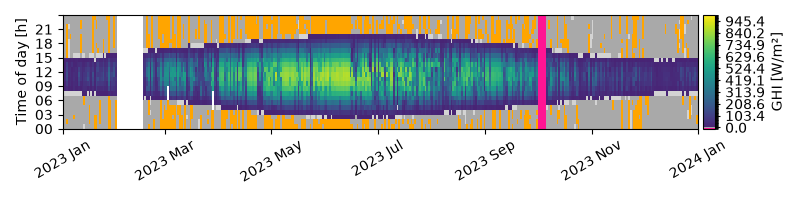
Advanced usage

With a few tweaks, the heatmap plots can be made much more informative. In particularly, using a custom colormap and overlaying sunrise and sunset times can make it easier to graps the data and detect data shifts.

The solarpy package has a custom colormap for solar irradiance data: solarpy.plotting.irradiance_colormap_and_norm(). The colormap uses a dark grey color for small negative offsets [-2, 0), orange for larger negative offsets [-6, -2), and a perceptually uniform colormap for positive values, with a maximum of 1000 W/m². A red color is used for unfeasible negative values, i.e., values below -6 W/m². This custom colormap makes it easy to assess thermal offsets and detect instrument changes.

The returned Axes can also be used to overlay additional information, such as sunrise and sunset times calculated with pvlib.solarposition.sun_rise_set_transit_spa.

In the example below, a synthetic data gap and an infeasible negative GHI value are introduced to demonstrate how these features can be visualised in the heatmap.

import solarpy
import pandas as pd
import matplotlib.pyplot as plt
import pvlib

# Introduce a synthetic data gap and an infeasible negative GHI value
data.loc["2023-02-01":"2023-02-15", "ghi"] = float("nan")
data.loc["2023-10-01":"2023-10-05", "ghi"] = -150

# Load custom colormap and norm
cmap, norm = solarpy.plotting.irradiance_colormap_and_norm(vmax=1000)

fig, ax = plt.subplots(figsize=(6, 3))

_ = solarpy.plotting.plot_intraday_heatmap(
    time=data.index,
    values=data["ghi"],
    cmap=cmap,
    norm=norm,
    colorbar_label="GHI [W/m²]",
    ax=ax,  # pass in existing axes
)

# Overlay sunrise and sunset times
sun_rise_set = pvlib.solarposition.sun_rise_set_transit_spa(
    pd.date_range(data.index.min(), data.index.max(), freq="1d"),
    meta["latitude"],
    meta["longitude"],
)

sunrise = (
    sun_rise_set["sunrise"] - sun_rise_set["sunrise"].index.normalize()
).dt.total_seconds() / 3600

sunset = (
    sun_rise_set["sunset"] - sun_rise_set["sunset"].index.normalize()
).dt.total_seconds() / 3600


ax.plot(sunrise, c="r", linestyle="dashed", lw=1.5, alpha=0.7)
ax.plot(sunset, c="r", linestyle="dashed", lw=1.5, alpha=0.7)

fig.tight_layout()

Notice in the advanced example, there is a very sharp line between daytime values and nighttime which makes it easy to detect time shifts in the data. Also, the custom colorbar makes it possible to quickly identify the magnitude of the nighttime thermal offsets, which in this example has quite some values in the range of -2 to -6 W/m², but no values below -6 W/m².

Timestamp resolution

The plotting function by default attempts to infer the time resolution of the data. If there is mixed timesteps, it is possible to override this paramter by setting the time_resolution parameter. The example below plots hourly data.

data_1h = data.resample("1h").mean()

fig, ax = solarpy.plotting.plot_intraday_heatmap(
    time=data_1h.index,
    values=data_1h["ghi"],
    time_resolution=60,  # 60 minutes = 1 hour
    cmap=cmap,
    norm=norm,
    colorbar_label="GHI [W/m²]",
)

fig.tight_layout()

Estimated memory usage: 335 MB